Geodatabases, Domains, Attributes

 Introduction:

Planning a collection of data points before entering the field can help properly collect data and allow concise collection of certain aspects. In this lab we discussed the development of geodatabases and its importance as a work space. The Geodatabase can also be a mobile platform that can be used both in lab and in the field by using the ArcPad Feature. This was utilized to collect data for microclimates. The implemanintation of geo databases in the field is important because it allows us to create domains and fields while away from a terminal that has access to ArcGIS or Catalog. This will allow us to be a mobile GIS platform.

The Mobile Platform:

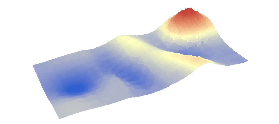
This lab focuses on microclimate data. A micro climate is a climate of a small or restricted area which differs from the surrounding area. A good example of this would be the wind speed is usually higher in a area that funnels the wind in creating a higher wind speed. To map this data we will have to be in the field for mobile collection. In order to collect in the field we have to use the Trimble Juno platform. This platform is useful since it has GPS based collection and can be integrated with Geodatabases that we create in the lab.

Methods:

The first step to getting ready for the field work is to create a Geodatabase in ArcCatolog. In ArcCatalog we created a file Geodatabase which is perferable for single or small work groups and is a cross platform system, which is useful since we will have to import this database to our Juno hand held units later.

After the database is completed we have to create Domains and fields. Domains are created in database and the fields are created in shapefiles. These two items can then be connected in ArcGIS to give attributes to the points that we collected. In ArcCatolog we have to think about what we want our domains to be.  This will help create the rules and legal values of the field type for enforcing data entry. For example we would want to have a short interger in for wind speed. Since the weather is also really nice out we would want to have a range of temperature to be relevenet to our collecting needs. This can be expressed as having a collection range of 20°F to 60°F, anything below or above will be ignored since this would be an error reading. Since we are collecting Microclimate data we will have to think about the what data we will collect. We decided to collect based on humidity, dew point, windspeed, temperature, and wind direction.

We are then ready to edit our domains with our selected data. To edit the domain we will have to right click on the file geodatabase and click properties. This will open the tab which contains the domain tab. We can then create the domain name and description. Also from this area we can select the type of data that can be entered in the field. The examples of this are text data, short interger, long interger or float. The last one is coded values. This can be coded with their own separate descriptions.  Once all our domains are set up we can move to ArcGis to complete the transfer of data.

Once in ArcGis we can begin to transfer the data over to the Trimble Unit. To do this we will have to activate the extension ArcPad Data Manger in the Extensions dropdown menu. We will then hit the button Get Data for ArcPad this will open up a wizard that will walk us through the entire process. Since we have our Geodatabase ready to go we can choose the menu Checkout all Geodtabase layers. This can also include a background image for reference, I howvere could not get a reference image to appear, this step however is purely optional. We can then change the file name of a folder that will store the data that is collected. I selected Micro_Kerraj for my storage area. The ArcPad manager will then create a ArcPad Map (.apm file) this file is what we will be using in the field for collection. Once this project is created we then create a backup folder incase something goes wrong, just to be safe.

To deploy this information on to the Juno unit we then just collect the GPS unit to the computer by using a USB, we will then go into the file system of the Juno and drag and drop the Micro_Kerraj folder that we created. We are now ready to go out and collect micro climate data. When we go out into the field we can see that the micro climate domains that we have created are visible and we have a range that we can follow. This helps the mapping process by allowing us to import a variety of data instantly that can be directly imported back into ArcGis.

Discussion:

Creating the Domains and the fields were easily handled but when I went to import a background image for reference nothing would work, since this step was optional I opted to leave it out of my final project. This however did make collection a bit more difficult since I had no bearing of where I truly was.  Importing a geodatabase to a hand held collection system is a simpler way then just simply going out and collecting points and collecting the data seperatly and combining them together later in ArcGIS. This field method allows for quicker data acquisition.

Conclusion:

GPS data collection with mapping GPS is different than just gathering a point. With the power of having a geodatabase behind the mapping unit we can give our points data instantly so that no additional steps would have to be taken when we import the data back into ArcGIS. This is also important since we will were doing proper data base setup before we left. If we were to accidently input -100°F in the Juno and we did not have the range set up we would have a huge outlier that could potentially skew our data. This is why it is important to have proper database setup and normalization and why this was an important project to learn.

Development of a Field Navigation Map

Introduction:



In order to navigate you need two sets of tools, the first has to be something to navigate with. Items that you can navigate with can be as simple as the sun or the North Star and can be as complicated as GPS otherwise known as a Global Positioning Satellite. The second needed tool is a from of location. This second tool is usually a map and can be combined with some sort of coordinate system and projection. Instead of using Lattitude and Longitude which is commonly found on small scale maps and globes we will be using UTM otherwise known as Universal Transverse Mercator coordinate system. We will also be using Geographic Coordinate System of Decimal Degrees. By using UTM and Decimal Degrees we will be able to create accurate maps for a large scale area.

UTM splits the world into a 2 dimensional cartesian coordinate system and divides the earth into sixy zones with a six degree band of longitude. This coordinate system was created by the US Army Corps. This is useful to use when original WGS 1984 becomes too large for the area. UTM can be used instead of WGS 1984 for a closer more in depth look at a specific area for our selected area we are using UTM zone 15.

Our second Coordinate system that was selected is NAD 1983 Wisconsin Transverse Mercator. This is similar to the UTM zone 15 but instead of having the longitudinal 90w to 96w it is specifically for the entire area of Wisconsin. With UTM zoning Wisconsin is split into zones 15 and 16 with NAD 1983 Wisconsin Transverse Mercator it is centered entirely in Wisconsin. This is useful when you need all of Wisconsin to be your area of study.


Methods:

To start the map we first had to create a pace count. With a pace count we can navigate a selected area using a map and compass. The pace will allow the user to measure 100 meters accurately by measuring how many paces it takes to traverse this distance, in my case it was 66 paces for 100 meters. This data will be used to map out and traverse the Priory study area

Creating a Map;

The project consisted of creating two functional maps for navigation. The first map consists of using the UTM System and the second will have the geographic coordinate system. To start we first had to import the data from the original source into a geodatabase of our own creation. In the data we have a topographic map, elevation data and a aerial photograph of the priory study area. I created a border around the priory area and extracted the elevation data by using the extract by mask tool. I then gave it a elevation scale that would be suitable for the project and used the clip tool to clip the 2ft contour lines to the area of study to create a map. for the grid I used a Degrees seconds map by 2 seconds for every tick in the grid. This map uses the Geographic coordinate system of NAD83



The second map was using the UTM zone 15 which is the zone where the priory falls under. to create this map I used the aerial photograph and the 5ft contour intervals. since this was not a raster I did not have to extract by Mask but instead used the clip tool to clip to the boundary with the aerial photograph. from this point I was able to use the 5ft contour interval lines to create a map. for the grid system I used a measured grid which uses meters instead of seconds. this grid system is set up with a tic every 75 meters.

Visualizing and Refining Terrain Survey Data

Introduction:

In the previous lab we worked on moving the data that we collected into a xyz table. This table however was not standardized. To normalize this data we have to go and create it into a basic xyz table with only three columns in excel. Normalizing data means adjusting the values measured on different scales to a notionally common scale. Where the intention is to bring the entire probably distributions of adjusted values into alignment. Our data points and how the interpolation procedure will help to visualize this data.

Methods:

First we have to normalize our data. To do this our group had to look at all the collected data and enter it into excel using only three columns. This allows us to interpolate correctly when we enter it into excel. When we enter the data into excel we have to create a new Geo database and import the xy table into this database so we can use the data we collected as a point system. After the data is imported we can begin interpolation.

Normalized table data

IDW is an acronym for inverse distance weighted technique. IDW is a spatial analyst function that determines cell values using a linearly weighted combination of a set of sample points. The weight is a function of inverse distance and the surface being interpolated should be that of a locational dependent variable. Ideally the more distant locations will have less of an influence on areas that are closer to other sample points.

Inverse Distance Weighted Interpolation

Natural Neighbors is an interpolation technique that applies weights to sample points based on proportionate areas to interpolate a value. By using an area that is near a point it will pass through that inputs sample and smooth everywhere except at locations of the input samples creating a fluid output.

Natural Neighbors Interpolation

Kriging is an interpolation technique that chooses to optimize smoothness of the fitted values. Kringing is used to give the best linear unbiased prediction of the intermediate values instead of the absolute max and min values that are inputted into Arc GIS

A sample of Kriging Interpolation, Ridge is not pronounced due to error in sampling

Spline is an interpolation technique that is a smoothing function, this is much like Kriging except it uses the absolute min and max inputs to create a smooth interpolation

A Sample of Spline Interpolation

TIN is short for triangulated irregular network. It is a digital data structure for the representation of a surface in a vector based representation of the physical land surface based on the xyz coordinates in polygonal triangles.

A sample of TIN interpolation

When we imported the data into Arcscene to get it to project properly we had to extort the data as a point feature class based on the xyz table so Arcscene could properly project in 3d. 

The results of the method are for the most part quit good however there are some places that need to be redone with a better more tight survey data. For example, the ridge was not projected correctly the group had to go back outside and redo this to create a better representation.

The Ridge has been re-sampled

Corrected Kringing, notice the ridge is better projected than the previous Kriging

This survey relates to other field based surveys because it is important how to learn how to use tools to create three dimensional locations based on data. This can be used in many different scenarios where models would have to be used before field data can be collected. This is important since models can be used to represent real world scenarios and can be based upon actual representations of the land before actual data points would be collected.

Results:

When we first imported into Arc Map the group was dismayed to find that the ridge feature was not projecting properly. To project this ridge properly we decided to go back out into the field to recollect points in a more dense fashion. When we re-projected the xyz table into ArcMap the ridge was finally being projected to an orientation that we were happy with.

Each interpolation technique is useful in their own way but for our project we decided to settle on Kriging since it give the most aesthetically pleasing map. The Kriging method also has the added bonus of averaging out the variables that we collected.

3D projection of Kriging with corrected Ridge

Summary:

This survey was useful to using detailed grid based survey methods to help collect points. Because the first survey was not accurate and didn’t collect all the points needed for the ridge part we had to go back out and recollect points. It was useful to see how the grid points can be used to easily collect data for Arc GIS. This was also a useful lab to see how we can go and re collect points that were skewed. With the grid system it was a snap to go back out and re collect data since we knew exactly where to go to collect. It was also interesting to see that interpolation can be used for elevation. This can be a powerful feature that can be used for other data besides elevation such as population density and income differences.

Creation of a Digital Elevation Suface Using Critical Thinking Skills and Improvised Survey Techniques

                As Geographers we are constantly looking for new and interesting ways to define the world and the environment that we live in. Geography is a huge subject that can encompass many different scientific practices. However each of these practices will have to follow basic rules to collect data. In the Geographic Field Survey course we are tasked with utilizing different methods of sampling techniques to create and collect data. By using our sampling systems correctly we will be able to utilize our time, energy, money, and man power effectively. Sampling will be used to collect data. The sampling methods that we will utilize can either be random, systematic or stratified. Random sampling is the best method to collect data without bias while systematic can collect data based on a set criteria. Stratified can be used with both random or systematic sampling but the areas in the field of interest must be known and must be quantitatively utilized in order to make stratified sampling useful.

                The objectives of this lab are to use a 2.34m x 1.12m sandbox to create five geomorphic models and utilize a grid system with a sampling method which will later be incorporated into a program such as Arc GIS or excel to create a three dimensional model of the collected data. In order to complete this survey we will have to create a spreadsheet of data with fields in X,Y, and Z.

Methods:

To complete the objectives the group decided to use snow to build the five geomorphic models. The models include a ridge, a large mountain, a valley, a depression and finally a plain area. In order to collect data from a sampling method the group used twine and thumbtacks to create a grid system which was 10cm x 10cm. This grid size will give us a  large area to work with and be very accurate with numerous sampling sizes. we opted to use a systematic sampling approach to collect data since it will be the best use of our time and resources.

Creating the study area

The grid will assign each square  its own x, and y value. To create the Z coordinate we went through each square and measured in cm to the wooden barrier around the sandbox. This was to be the sea level. While two people measure the Z coordinate in each grid one person had a spreadsheet created with labeled areas to create a quantitative graph of each area which would be later incorporated into a excel sheet.

Results:

The resulting numbers of the 10cm x 10cm grid were numerous. To create a good sampling system we are supposed to have a great number of samples since the x value is 23 by a y or 11 we collected a total of 242 samples to give us a good sampling base.

The Grid system is built and ready to collect data

 The minimum sample collected was -17.5 and the maximum was 20 when we look at a color coded excel sheet we can begin to notice a pattern in the data already with the ridge and the mountain becoming evident on the placement in the grid system as positive areas and the depression and valley as negative. With this data it will be very interesting to see the final product when we incorporate it into Arc GIS for a full three dimension look at the data

Conclusion:

In conclusion we were able to create a spatial model by thinking critically and using the data and equipment that was provided to us. By using a grid system in a 10cm x 10cm format we were able to create and collect a satisfying amount of data by using a systematic sampling method which can be used later in excel and Arc GIS. 

Collected data shows the ridge, mountain, valley and depression