Navigation using UTM coordinate Maps

Introduction:

The previous lab from February had the students create maps based on UTM gridsthat had a navigation function using paces that were taken from a measured area. This data was then inserted into a map that would then be used for navigation in the field. Using these field maps in the area of study it was possible to use GPS and the created maps to find and collect points that were assigned to the group.

Area of Study:
The area of study is the Priory. The Priory is a UWEC returning student housing area for non traditional students. It was originally a priory for monks before it was re purposed for student housing. This is a residence hall that is set in 120 acres of woods that is inter-cut with semi moderated trails. Since this area is in the wilderness with a large area of woods it is easy to get lost and difficult to traverse.

Methods:
The original maps that were created in February were used to navigate the priory. before setting forth and collected the GPS coordinates onto a GPS device it was important to record the area that was hiked along the way. The GPS that was utilized has a function to switch from Lat and Long to UTM grid system. This was used to correspond to the maps that were originally created. It was at this point that we would have to find a way to prove we made it to the UTM points that were assigned to the group. This was accomplished by collecting a point in the GPS unit and by taking a picture that had location enabled. once the initial set up is completed the group decided to plot the assigned points onto the map to create a ease of access and navigation area. This was sort of a rudimentary navigation chart.

UTM Grid Map used (credit Rachel Hopps)

Once the initial set up was complete with the GPS unit and the map it was time to navigate to the points plotted. At the start up the group decided that it would be best to stick to areas that looked like they had a trail attached. This allowed the group to move from trail to point in a quick succession. However some points were located deep in the woods. to move quickly from point to point we jumped as fast as possible from point to point by going in as straight as lines as possible. This was difficult because of the heavy vegetation in some areas that forced the group to take drastically different directions in order to navigate the area which can be seen on the tracking data.

Collecting the first point with Rachel and Joseph

After the points were collected it was time to update the area in order to create a map. To do this we had to use the GPS number that was attached to the unit and the group number that was assigned in order to get the data. once the data was inserted into ArcGIS it was possible to see how well the group traversed the area.

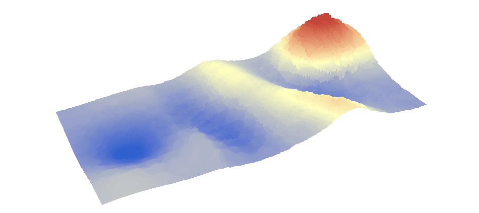
One known problem that the group noticed is that the compass on the GPS was not the greatest for quick turn around. The compass is electronic and would take a few moments to adjust to the direction of the group. This made travel frustrating as the group would have to re adjust every 10 meters or so. Other sources of frustration came from the heavy amounts of vegetation and brambles about. The vegetation made travel difficult and with the brambles, sometimes painful. The map also did not contain some data that would be useful to the group. The data that would have been useful to the group would have been elevation data in the form of topographic maps since some of the points were in an elevated position this data would be useful and should not have been excluded

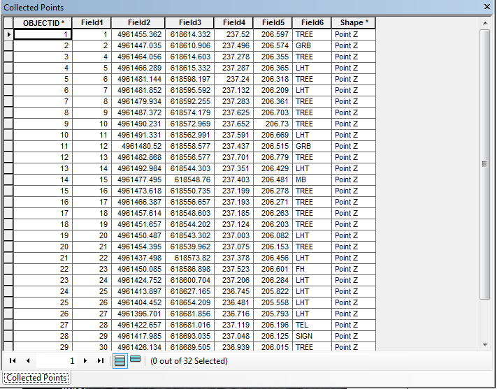
Tracking Path and collected coordinates

Results: 

For the majority of the experience we can see that the group made short work of the points with only a couple of instances where the point collected was difficult to traverse to. this is because the initial planning allowed the group to plan an approach as well as having a set job for each person. one person would be using the GPS unit for measuring the tracking and navigating with a compass, another would be using the UTM map to geed the coordinates that were needed to the GPS user and to count pace. The third and last person would be breaking the trail up for ease of travel and would take pictures and notes. By using a three person team it was possible to create a sort of oblong circle to collect all the points which were then inserted into ArcGIS

Conclusion: 

Collecting data in the field is the prime example of geography. Some agencies require field methods and the ability to create a accurate map and to use the GPS and UTM coordinate map created for a Area of study is invaluable for many companies and profiles. This area of study and map creation and field navigation is useful for surveying, search and rescue and many other applications. 

Processing UAS Data in Pix4D

Processing UAS data in Pix4D

The Pix4D software is a Drone Mapping Software for professional drone based mapping purely from images that are taken with an aerial mapping platform. It is possible to use the Pix4D software to create cutting edge results that include but are not limited to Thermal mapping and 3D mapping. It is a useful software that is used in a variety of industries including emergency response, agriculture, mining and real estate. It is a easy to use program that almost anyone can pick up and enjoy.

How to use Pix4D:

Before starting a project it is important to have a image acquisition plan. This is an important step to create keypoints. Key points are a characteristic point found in an image. When 2 key points on 2 different images are found to be the same they are called matched key points, each match Key point will produce a 3D point. The more points captured the more accurately 3D points will be computed. So a high overlap of images is required, at the very least 75% frontal overlap and 60% side overlap is needed. If the user is flying over a homogeneous area such as sand/snow or a uniform field like agriculture lands it is important to increase the overlap to the images by at least 85% frontal overlap and 70% side overlap. Flying higher will also improve the results as well as having accurate image geolocation available.  An available tool for use is rapid check, rapid check is used to verify the proper ares and coverage of a data collection. The Pix4D software is also able to process multiple flights. The pilot does need to make sure that each plan captures the images with enough overlap and that there is enough overlap between the 2 image acquisition plans under the same weather conditions. It is also important that the flight height should not be too different between the flights since this can change the spatial resolution.

In order to produce oblique images the type of data that we need to take is the GSD or Ground sampling distance. It is advised to create Ground Control Points (GCP) if no GCP are used than the scale and orientation constraints can be used. If neither GCPs or constraints are used the final result will have no scale, orientation and no absolute position information. This will make it impossible to use for measurements, overlay and comparison. Finally when the process runs through the Pix4D system we will get a quality report which will report the information computed during the process. This will give us information regarding how many points were acquired the amount of overlay obtained and a summary of the project which can have the AGD, and the amount of area covered.

Methods: 

To use the software we will have to import images that were captured with a UAV device. this could be a multi bladed copter or a fixed winged UAV. After the initail mission is completed and it is time to import the data into Pix4D w must use the Project selection tool. this will import all the data into the program to utilize for later. 

After we select the image properties and where the output file will be located it is time to run the Pix4D program. The Pix4D program to find areas where overlaying occurs and will draw points data and create a area that can be used for three dimensional analysis. 

When the initial process is completed we can then complete a point cloud mesh and create a DSM orthomosaic with indexing. this process takes a long time to complete so it is best to set the program to run and then grab dinner or complete other required work. After the completion of the Point cloud and Mesh with the DSM and Orthomosaic index we then have a completed area that can be used for a variety of other useful applications such as three dimensional maps.

 What is left after the indexing is a summary of what has been completed this holds a varity of information such as the total amount of points collected. The completed GSD and the total area that is covered. what is also completed in the program is a wire mesh of the area selected. 

Conclusion:

The pix4d program is a intense program that can be useful to the geographer who is using the UAV for mapping purposes. by using overlaying pictures it is possible to create a three dimensional map that can be later used for a variety of applications including areas that are quite large. the amount of accuracy that can be utilized is also impressive considering that the amount of time to fly a UAV to the selected area and take the amount of pictures required only needs a small amount of time in relation to how it would be to do the same thing manually. Pix4D is an impressive tool that can be utilized to great extent in areas such as surveying, evacuation data and medical and emergency services.

Topographic Survey with total station

Introduction:

In the previous entry RTK GPS Unit was utilized to create accurate point collections. In this week we are using the RTK GPS Unit again but with some added surveying equipment. The Topcon Total Station and the Prism Laser collector. This is a useful application that is similar to the previous activity of the Distance/ Azimuth survey methods. The Major difference between the Distance/Azimuth survey and the Total Station survey methods is that this does the same surveying job but much better. This method will be used to survey points by using the total station for later use in building a micro topographic surface with the points that we have collected.

How Total Station works using Geographic Origin.

Methods:

Setting up the Topographic Survey and Total Station

This topographic Survey with total station was a group effort with another partner since one person needs to be in charge of the Prism mechanism and one person needs to enter the points into the RTK GPS Unit. Classmate Luke Prashak was here to assist in the collection of points.

To begin the setup of the RTK, Prism, and Total Station needs to be located and set into a correct designated static position. This position is called the static point or the occupied point. To correctly set up the static position of the total station due north needs to be found. This will then be taken with points that were set up with orange flags. By using the orange flags as backsight points we can now know the exact static point via the prism collection based on collecting the information on the orange flags. Because this system is dependent on mm accuracy we cannot touch the total station once it is set into the static position.

 Prof. Hupy in the field with Total Station and RTK unit 

The first step is to gather the backsights which are BS1, BS2 etc. Once the backsights are collected it is time to gather the occupied point where the Total Station will reside. In order to set up the TSS we have to ensure that the surface is clean and dirt free. After the surface is cleaned, extend all three legs equally and secure the locking mechanism for a sturdy base for the tripod. Once the base is set centered attach the tripod head over the point while remaining level. A good way to ensure centering is to drop a pebble from the center of the tripod head. Then step down firmly on the footpads to set the legs into position.

The instruments are next to set up. Center the tripod head and secure the instrument to the tripod and bring all the leveling screws to the natural position below the line on the screw post. From here look through the optical plummet for parallel and focus on the ground. With the laser plummet on, position the instrument directly over point by using leveling screws. Be sure to observe what two legs need to be adjusted to bring the bubble into the middle and do not move the third leg. Release the horizontal tangent lock and rotate the instrument until tubular level is parallel. Once everything is centered and level it is time to recheck the fine (tubular) bubble vial in position 1 and 2 and adjust as needed. If no adjustments are needed then measurements can begin to be made.

To take points we need to turn on the total station and switch on the Bluetooth which is located in the parameters portion in order for the Tesla to recognize it. Now it is possible to connect the RTK to Total Station. To begin the OCC/BS Set up go to the Home Screen for Magnet and select the Setup icon and then select the backsight icon. Enter all the needed information for the total station and for the Prism Rod. It is very important to keep the prism rod at the same measurements throughout the point capturing. If the rod needs to be moved it will have to be recorded in the Total Station that the prism was moved or it will throw the data collected and will not be nearly as accurate. Finally place the prism rod over the backsight point and gather the point. This is needed to zero out the total station for due North. Collect the GPS points with the Tesla in Magnet Using the total Station and Prism in the Survey icon screen.

Collection of Points with RTK and Total Station
The system is now ready to collect points. Looking through the viewfinder on the total station it is imperative to lock onto the prism system. After locating the prism system on the Total Station it is then possible to use the view finder to manually focus in on the prism. at the ranges we were dealing with the magnifier was not necessarily needed but it was useful to practice. We are then ready to collect the point, Signaling the person manning the RTK will then collect the point after a series of seconds the point is then collected and we can move on to the next adjacent point. The points collected will be used with additional points to later be imported into ArcGis and create a topographic map. 

Creating the map in ArcGis 

By using the data imported from the RTK and Total station in a .txt format it is possible to use the create feature tool from xy table and import the points into ArcMap. From here it is possible to use these points to create a IDW (inverse distance weighted) analysis which would include the z axis. IDW uses every point collected to create a raster that will give the analysis of height. To use this tool  import the xy and z data into the tool and then run the analysis. From this data the height is now mapped in a topographic manner. The lower the point will be green the higher the point will be red. 

Results: 
From the IDW the green points are the lower collected areas that are taken in the little Niagra river area and the higher points are the areas that are collected above the geographic origin point which is where the total station was located. This is an important tool in mapping areas that require height to be accurate to the nearest millimeter. 

collected points interpolated with IDW 

Conclusion: 
By using Total Station and RTK we can map areas with the greatest of accuracy. This is an important tool when using drones is either illegal or ill advised. The IDW tool is useful in creating a topographic map that can be used for analysis in other areas. 

Surveying of Point Features Using Duel Frequency GPS

In order to create a topographic map it is imperative to understand the Dual Frequency GPS equipment.

In order to do this we have to know what a dual frequency receiver does. This is a signal capturing system that can select and simultaneously receive signals on two frequency channels during a specific time period. This is a good system to use to gathering point data that is incredibly accurate and can accurately gather points to within a centimeter of where they were taken. In this introductory lesson we learned how to take different points and then use the data to create a map in ArcGIS.

 RTK Unit 

The study area that we have selected was the area that is outside of Davies and UWEC Phillips Science Hall. This area allowed us to collect numerous different points such as trees, garbage cans, and light polls. This was useful as an introductory course in the Surveying. The surveying equipment utilized is the RTK GPS Unit. RTK stands for Real Time Kinematic. It is used for extremely high accurate positional accuracy by using a consistent connection to the internet via Wi-Fi. Every time we collect a point using the RTK GPS Unit it collects 30 points and averages all of them out. This allows for extremely accurate data collection.

RTK Unit Screen 

When collected there is also XYZ data from the GPS unit. This can then be used in ArcGIS by selecting the tool import XY and map out the points in ArcGIS. The points can then be redone in ArcMap by selecting the projection which is UTM zone 16. The XYZ data can then be used to map where the points will be located. From here it was simply selecting the points in the attribute table by what they were in the definition which was entered into the GPS unit upon capture. From here it is simple to use this data to create a basic survey map.

The results of this data show very accurate GPS collected points using the RTK GPS Unit. This is a useful tool for surveying points that require accurate information. An example of this would be road surveying and forestry work. The results of the captured points are incredibly accurate. This RTK GPS Unit also has the added benefit of allowing us to input attribute data directly on capture versus where it would be necessary to know what to capture before surveying with other equipment.  

Collected Survey Points 

To conclude the RTK is a useful tool when accuracy is important to the application at hand. The only downside is that this a large unit and is slightly cumbersome to carry around everywhere. The GPS unit is also great since it allows on the fly attribute creation. Overall this is a very useful tool that I look forward to working with in the future. 

Distance and Azimuth Surverying

Conducting a distance Azimuth survey

Introduction: surveying with a grid based coordinate system is good on small plots but it is not ideal for many geographic circumstances. These days you can use GPS technology along with survey stations but sometimes you cannot rely on technology to come through. This is why distance and azimuth can come into play. It is a very basic technique that can work on many different conditions that can rely on sampling techniques and point quarter method. This allows us to map out linear features on a landscape from a singular point based on the azimuth of where the point was taken using the tools in ArcGIS such bearing distance to line command and feature vertices to points command. In this exercise we looked at the tree density in Putnam Park.

Azimuth Surveying in quadrants from Origin

Study Area:

The area of study for this assignment is the Putnam park area of the University of Eau Claire. In this area are new and old trees that have been planted on the grounds of the University of Eau Claire. This area is a good step for Azimuth surveying as it allows for a variety of tree species to be mapped with differing diversity and density. We will be collecting 10-20 point-quarter data collection of these locations from a centralized location that will not change.

Survey Area: Putnam Park 

Methods:

The first step in Azimuth surveying is to do the research of azimuth surveying. Azimuth surveying is an angular measurement in a spherical coordinate system that looks at the vector from an origin point which is then projected onto a reference plane. The angle between the projected vector and the reference vector is called the azimuth. An example is the North Star. The origin point can be the person looking at the point and the azimuth would be the angle between the North Star, the surface of the ground and the perpendicular projection of the ground. This can then be measured in degrees and can then be used in mapping. This is an older style of mapping without the use of relying on technology.

 Although we still rely on the technology in the form of the True Pulse 360 B.

Once we have the 360 B true pulse set up in an origin point in Putnam Park it is time to begin to take points. We are looking at trees and the azimuth of the trees as well as the distance from the point. To collect the distance we will be using a laser pathfinder and will relay the information back to the True Pulse system. This will allow use to laser designate the distance between the origin point and the point that we are collecting, this means we only have to use one latitude and longitude point which will be the origin station.

True Pulse 360 B 

After the points are collected it is time to import the data into an excel spreadsheet. The XY will be the same for all the points right now. When we enter the excel table we are adding in the diameter the azimuth, distance and tree type. From here we connect the excel table to the blank map in arcgis.

We will then convert the excel table to a usable format in arc catalog by adding the data into a geodatabase which we can then use the xy table from the excel sheet and create a point based on the xy data. It is important to mark the xy table correctly otherwise the next tools will not work. When the data was imported into excel the xy data was flipped so the Y coordinates were actually the X coordinates and the X coordinates were the Y coordinates. This meant that the data could not be used until it was corrected.

XY Data

Once this data is converted into a single point we can then run the tool bearing distance to Line command in the features tool set which creates a new feature class containing the geodetic line features constructed based on the values in a xy coordinate field as well as the distance field of the table. This will create only lines from the origin point. It is important to note that since this is a broad service WGS 1984 coordinate system needs to be utilized to make accurate readings.

Since the Bearing Distance to Line Command only creates lines from the origin point we will have to use the Feature Vertices to Points command in the features tool set to create actual points at the end of the lines. This will allow us to use the data that we collected by creating a feature class generated from the vertices of the lines. In essence it will create point data at the end of our line data.

Results:

The results of using Azimuth surveying are extremely accurate. This is a useful tool that is still in use today. It allows highly accurate data to be accumulated and does not rely on GPS or other highly advanced technology. This means that because the technology is not present it has a higher risk of not failing. The results from this azimuth survey are impressive and show that from a single origin point we can collect data that can be used for a multitude of purposes including road surveys, tree surveying and logging expeditions.

Conclusions:

Because technology can sometimes be a hindrance in field work it is important to rely on older more trusted methods like Azimuth surveying. If data needs to be collected in heavy foliage which would normally interfere with GPS systems Azimuth surveying could be used instead to create accurate maps. This is why Azimuth mapping is still used heavily for surveying work such as road construction and tree surveying. 

Arc Collector: Gathering Geospatial data on a Android Smartphone

Introduction:

In the previous post the method of collecting points and data used a dedicated platform known as ArcPad. This is a good method when you have a dedicated system and technology to run smoothly with ESRI technology. However in the modern era most people carry around a smart phone or a tablet device. These devices can have many times more computing power than GPS units and would be useful to use as collection devices. This is where the ArcCollector app comes in. it is a software app that works with ESRI and ArcMap to gather data on the fly using commonly found IOS software and Droid software.

image source: http://resources.arcgis.com/en/communities/smartphone-apps/

Study Area:

The study area that we selected is the same as the Arc Pad study area. We are also using the same criteria in our collection points. The collection points include wind speed, wind direction, relative humidity, temperature and dew point. To complete the objective of the lab the class was broken into separate groups to collect points in their retrospective area to merge together later.


Methods:

The first step to using Arc Collector is downloading it onto the smartphone or tablet device. Once the app is downloaded we will have to connect it to the UWEC arcgisonline profile. This is the hub where we will be storing and collecting our data which can then be deployed to ArcMap for further modification. It was important to login using our Enterprise account so we can have access to the majority of the online functions that ESRI provides as well as have a online profile to transfer and modify data that we have collected. From the ArcGisonline account we can then deploy our project simply by going to the my content page and selecting the profile in which we will be deploying. ArcGISonline is also useful for editing the meta data of the project such as tags, editing, exportation of data and synchronization.  For this project I have selected  Microclass_Kerr to collect points to deploy as a web map. We already had the Geodatabase, domains, and feature classes created so this was useful to save time in our project.

To deploy our points we simply select what we would like to deploy to our device from our handheld smart phone. once the data has uploaded onto the smartphone or tablet the group could then exit the lab and being to collect points. To collect points we used various tools such as compasses to gather data relating to wind direction, and a digital monitor to measure the temperature and humidity. Two group members continued to gather 20 points in the study area to gather a total of 40 points giving us a large sample size that can later be imported into ArcGIS. Once all the points are collected they can be saved and with a strong wireless connection as long as the synchonization tab was selected in ArcGIS online. We would then be able to automatically update our map. From this point we just have to select the option "Open in ArcGIS for desktop" to complete our transition to ArcMap.

ArcCollector as seen on the Droid device. 

Once our points were downloaded to Arcmap we uploaded our own set of points to a share folder. The other group members did the same and importing their points to our system was a breeze. The points were then imported to our own map which can then be edited into a functional map showing micro climates in the University of Wisconsin Eau Claire area.

Results:

The results of the collected micro climate points show varying differing temperatures that affect UWEC campus. This data is useful since the climate of Eau Claire can be different depending on the area where a person may be. for example, it may be more windy in one section such as the bridge area which can then be a cooler climate. To look more in depth about the various temperatures  I created a Hotspot Analysis of where the hotter and cooler temperatures are taken. higher temperatures are centered around areas that get more direct sunlight and where heat isn't as absorbed from plant life and is reflected by buildings and roads. This is a simple map to show case the ArcCollector abilities and should not be taken as scientific fact.

Hotspot analysis of Microclimate temeratures with points collected by ArcCollector

The data that was collected using ArcCollector is useful to use since the points are collected all at the same time with different group members, this is a useful tool since gathering points with more people will cut the time down from a multi day project to a mere couple of hours.


Conclusions:

The ArcCollector app is a powerful tool in the geographers arsenal. it can be used with almost anyone that has a IOS or Droid device and does not rely on propitiatory software. This is also a useful app for collecting purposes since the data is seamlessly synchronized directly back to the registered online ArcGIS profile. The benefits of using ArcCollector over ArcPad are staggering. because of the ease of use and the quality of the maps that were created I would highly suggest using ArcCollector instead of ArcPad.

Geodatabases, Domains, Attributes

 Introduction:

Planning a collection of data points before entering the field can help properly collect data and allow concise collection of certain aspects. In this lab we discussed the development of geodatabases and its importance as a work space. The Geodatabase can also be a mobile platform that can be used both in lab and in the field by using the ArcPad Feature. This was utilized to collect data for microclimates. The implemanintation of geo databases in the field is important because it allows us to create domains and fields while away from a terminal that has access to ArcGIS or Catalog. This will allow us to be a mobile GIS platform.

The Mobile Platform:

This lab focuses on microclimate data. A micro climate is a climate of a small or restricted area which differs from the surrounding area. A good example of this would be the wind speed is usually higher in a area that funnels the wind in creating a higher wind speed. To map this data we will have to be in the field for mobile collection. In order to collect in the field we have to use the Trimble Juno platform. This platform is useful since it has GPS based collection and can be integrated with Geodatabases that we create in the lab.

Methods:

The first step to getting ready for the field work is to create a Geodatabase in ArcCatolog. In ArcCatalog we created a file Geodatabase which is perferable for single or small work groups and is a cross platform system, which is useful since we will have to import this database to our Juno hand held units later.

After the database is completed we have to create Domains and fields. Domains are created in database and the fields are created in shapefiles. These two items can then be connected in ArcGIS to give attributes to the points that we collected. In ArcCatolog we have to think about what we want our domains to be.  This will help create the rules and legal values of the field type for enforcing data entry. For example we would want to have a short interger in for wind speed. Since the weather is also really nice out we would want to have a range of temperature to be relevenet to our collecting needs. This can be expressed as having a collection range of 20°F to 60°F, anything below or above will be ignored since this would be an error reading. Since we are collecting Microclimate data we will have to think about the what data we will collect. We decided to collect based on humidity, dew point, windspeed, temperature, and wind direction.

We are then ready to edit our domains with our selected data. To edit the domain we will have to right click on the file geodatabase and click properties. This will open the tab which contains the domain tab. We can then create the domain name and description. Also from this area we can select the type of data that can be entered in the field. The examples of this are text data, short interger, long interger or float. The last one is coded values. This can be coded with their own separate descriptions.  Once all our domains are set up we can move to ArcGis to complete the transfer of data.

Once in ArcGis we can begin to transfer the data over to the Trimble Unit. To do this we will have to activate the extension ArcPad Data Manger in the Extensions dropdown menu. We will then hit the button Get Data for ArcPad this will open up a wizard that will walk us through the entire process. Since we have our Geodatabase ready to go we can choose the menu Checkout all Geodtabase layers. This can also include a background image for reference, I howvere could not get a reference image to appear, this step however is purely optional. We can then change the file name of a folder that will store the data that is collected. I selected Micro_Kerraj for my storage area. The ArcPad manager will then create a ArcPad Map (.apm file) this file is what we will be using in the field for collection. Once this project is created we then create a backup folder incase something goes wrong, just to be safe.

To deploy this information on to the Juno unit we then just collect the GPS unit to the computer by using a USB, we will then go into the file system of the Juno and drag and drop the Micro_Kerraj folder that we created. We are now ready to go out and collect micro climate data. When we go out into the field we can see that the micro climate domains that we have created are visible and we have a range that we can follow. This helps the mapping process by allowing us to import a variety of data instantly that can be directly imported back into ArcGis.

Discussion:

Creating the Domains and the fields were easily handled but when I went to import a background image for reference nothing would work, since this step was optional I opted to leave it out of my final project. This however did make collection a bit more difficult since I had no bearing of where I truly was.  Importing a geodatabase to a hand held collection system is a simpler way then just simply going out and collecting points and collecting the data seperatly and combining them together later in ArcGIS. This field method allows for quicker data acquisition.

Conclusion:

GPS data collection with mapping GPS is different than just gathering a point. With the power of having a geodatabase behind the mapping unit we can give our points data instantly so that no additional steps would have to be taken when we import the data back into ArcGIS. This is also important since we will were doing proper data base setup before we left. If we were to accidently input -100°F in the Juno and we did not have the range set up we would have a huge outlier that could potentially skew our data. This is why it is important to have proper database setup and normalization and why this was an important project to learn.

Development of a Field Navigation Map

Introduction:



In order to navigate you need two sets of tools, the first has to be something to navigate with. Items that you can navigate with can be as simple as the sun or the North Star and can be as complicated as GPS otherwise known as a Global Positioning Satellite. The second needed tool is a from of location. This second tool is usually a map and can be combined with some sort of coordinate system and projection. Instead of using Lattitude and Longitude which is commonly found on small scale maps and globes we will be using UTM otherwise known as Universal Transverse Mercator coordinate system. We will also be using Geographic Coordinate System of Decimal Degrees. By using UTM and Decimal Degrees we will be able to create accurate maps for a large scale area.

UTM splits the world into a 2 dimensional cartesian coordinate system and divides the earth into sixy zones with a six degree band of longitude. This coordinate system was created by the US Army Corps. This is useful to use when original WGS 1984 becomes too large for the area. UTM can be used instead of WGS 1984 for a closer more in depth look at a specific area for our selected area we are using UTM zone 15.

Our second Coordinate system that was selected is NAD 1983 Wisconsin Transverse Mercator. This is similar to the UTM zone 15 but instead of having the longitudinal 90w to 96w it is specifically for the entire area of Wisconsin. With UTM zoning Wisconsin is split into zones 15 and 16 with NAD 1983 Wisconsin Transverse Mercator it is centered entirely in Wisconsin. This is useful when you need all of Wisconsin to be your area of study.


Methods:

To start the map we first had to create a pace count. With a pace count we can navigate a selected area using a map and compass. The pace will allow the user to measure 100 meters accurately by measuring how many paces it takes to traverse this distance, in my case it was 66 paces for 100 meters. This data will be used to map out and traverse the Priory study area

Creating a Map;

The project consisted of creating two functional maps for navigation. The first map consists of using the UTM System and the second will have the geographic coordinate system. To start we first had to import the data from the original source into a geodatabase of our own creation. In the data we have a topographic map, elevation data and a aerial photograph of the priory study area. I created a border around the priory area and extracted the elevation data by using the extract by mask tool. I then gave it a elevation scale that would be suitable for the project and used the clip tool to clip the 2ft contour lines to the area of study to create a map. for the grid I used a Degrees seconds map by 2 seconds for every tick in the grid. This map uses the Geographic coordinate system of NAD83



The second map was using the UTM zone 15 which is the zone where the priory falls under. to create this map I used the aerial photograph and the 5ft contour intervals. since this was not a raster I did not have to extract by Mask but instead used the clip tool to clip to the boundary with the aerial photograph. from this point I was able to use the 5ft contour interval lines to create a map. for the grid system I used a measured grid which uses meters instead of seconds. this grid system is set up with a tic every 75 meters.

Visualizing and Refining Terrain Survey Data

Introduction:

In the previous lab we worked on moving the data that we collected into a xyz table. This table however was not standardized. To normalize this data we have to go and create it into a basic xyz table with only three columns in excel. Normalizing data means adjusting the values measured on different scales to a notionally common scale. Where the intention is to bring the entire probably distributions of adjusted values into alignment. Our data points and how the interpolation procedure will help to visualize this data.

Methods:

First we have to normalize our data. To do this our group had to look at all the collected data and enter it into excel using only three columns. This allows us to interpolate correctly when we enter it into excel. When we enter the data into excel we have to create a new Geo database and import the xy table into this database so we can use the data we collected as a point system. After the data is imported we can begin interpolation.

Normalized table data

IDW is an acronym for inverse distance weighted technique. IDW is a spatial analyst function that determines cell values using a linearly weighted combination of a set of sample points. The weight is a function of inverse distance and the surface being interpolated should be that of a locational dependent variable. Ideally the more distant locations will have less of an influence on areas that are closer to other sample points.

Inverse Distance Weighted Interpolation

Natural Neighbors is an interpolation technique that applies weights to sample points based on proportionate areas to interpolate a value. By using an area that is near a point it will pass through that inputs sample and smooth everywhere except at locations of the input samples creating a fluid output.

Natural Neighbors Interpolation

Kriging is an interpolation technique that chooses to optimize smoothness of the fitted values. Kringing is used to give the best linear unbiased prediction of the intermediate values instead of the absolute max and min values that are inputted into Arc GIS

A sample of Kriging Interpolation, Ridge is not pronounced due to error in sampling

Spline is an interpolation technique that is a smoothing function, this is much like Kriging except it uses the absolute min and max inputs to create a smooth interpolation

A Sample of Spline Interpolation

TIN is short for triangulated irregular network. It is a digital data structure for the representation of a surface in a vector based representation of the physical land surface based on the xyz coordinates in polygonal triangles.

A sample of TIN interpolation

When we imported the data into Arcscene to get it to project properly we had to extort the data as a point feature class based on the xyz table so Arcscene could properly project in 3d. 

The results of the method are for the most part quit good however there are some places that need to be redone with a better more tight survey data. For example, the ridge was not projected correctly the group had to go back outside and redo this to create a better representation.

The Ridge has been re-sampled

Corrected Kringing, notice the ridge is better projected than the previous Kriging

This survey relates to other field based surveys because it is important how to learn how to use tools to create three dimensional locations based on data. This can be used in many different scenarios where models would have to be used before field data can be collected. This is important since models can be used to represent real world scenarios and can be based upon actual representations of the land before actual data points would be collected.

Results:

When we first imported into Arc Map the group was dismayed to find that the ridge feature was not projecting properly. To project this ridge properly we decided to go back out into the field to recollect points in a more dense fashion. When we re-projected the xyz table into ArcMap the ridge was finally being projected to an orientation that we were happy with.

Each interpolation technique is useful in their own way but for our project we decided to settle on Kriging since it give the most aesthetically pleasing map. The Kriging method also has the added bonus of averaging out the variables that we collected.

3D projection of Kriging with corrected Ridge

Summary:

This survey was useful to using detailed grid based survey methods to help collect points. Because the first survey was not accurate and didn’t collect all the points needed for the ridge part we had to go back out and recollect points. It was useful to see how the grid points can be used to easily collect data for Arc GIS. This was also a useful lab to see how we can go and re collect points that were skewed. With the grid system it was a snap to go back out and re collect data since we knew exactly where to go to collect. It was also interesting to see that interpolation can be used for elevation. This can be a powerful feature that can be used for other data besides elevation such as population density and income differences.

Creation of a Digital Elevation Suface Using Critical Thinking Skills and Improvised Survey Techniques

                As Geographers we are constantly looking for new and interesting ways to define the world and the environment that we live in. Geography is a huge subject that can encompass many different scientific practices. However each of these practices will have to follow basic rules to collect data. In the Geographic Field Survey course we are tasked with utilizing different methods of sampling techniques to create and collect data. By using our sampling systems correctly we will be able to utilize our time, energy, money, and man power effectively. Sampling will be used to collect data. The sampling methods that we will utilize can either be random, systematic or stratified. Random sampling is the best method to collect data without bias while systematic can collect data based on a set criteria. Stratified can be used with both random or systematic sampling but the areas in the field of interest must be known and must be quantitatively utilized in order to make stratified sampling useful.

                The objectives of this lab are to use a 2.34m x 1.12m sandbox to create five geomorphic models and utilize a grid system with a sampling method which will later be incorporated into a program such as Arc GIS or excel to create a three dimensional model of the collected data. In order to complete this survey we will have to create a spreadsheet of data with fields in X,Y, and Z.

Methods:

To complete the objectives the group decided to use snow to build the five geomorphic models. The models include a ridge, a large mountain, a valley, a depression and finally a plain area. In order to collect data from a sampling method the group used twine and thumbtacks to create a grid system which was 10cm x 10cm. This grid size will give us a  large area to work with and be very accurate with numerous sampling sizes. we opted to use a systematic sampling approach to collect data since it will be the best use of our time and resources.

Creating the study area

The grid will assign each square  its own x, and y value. To create the Z coordinate we went through each square and measured in cm to the wooden barrier around the sandbox. This was to be the sea level. While two people measure the Z coordinate in each grid one person had a spreadsheet created with labeled areas to create a quantitative graph of each area which would be later incorporated into a excel sheet.

Results:

The resulting numbers of the 10cm x 10cm grid were numerous. To create a good sampling system we are supposed to have a great number of samples since the x value is 23 by a y or 11 we collected a total of 242 samples to give us a good sampling base.

The Grid system is built and ready to collect data

 The minimum sample collected was -17.5 and the maximum was 20 when we look at a color coded excel sheet we can begin to notice a pattern in the data already with the ridge and the mountain becoming evident on the placement in the grid system as positive areas and the depression and valley as negative. With this data it will be very interesting to see the final product when we incorporate it into Arc GIS for a full three dimension look at the data

Conclusion:

In conclusion we were able to create a spatial model by thinking critically and using the data and equipment that was provided to us. By using a grid system in a 10cm x 10cm format we were able to create and collect a satisfying amount of data by using a systematic sampling method which can be used later in excel and Arc GIS. 

Collected data shows the ridge, mountain, valley and depression